What Causes Measurement Errors?
Now that we know the types of measurement errors that can occur, what factors lead to errors when we take measurements? We can separate this category into 2 basic categories: instrument and operator errors. Human errors are not always blunders however since some mistakes are a result of inexperience in trying to make a particular measurement or trying to investigate a particular problem.
Even if we know about the types of error we still need to know why those errors exist. We can break these into two basic categories: Instrument errors and Operator errors.Instrument Errors
When you purchase an instrument (if it is of any real value) it comes with a long list of specs that gives a user an idea of the possible errors associated with that instrument. In labs as a faculty you may be using equipment that is not new, so you should help students be aware of the errors associated with the instrument. If the company that made the instrument still exists you can contact them to find out this information as well. Looking at these carefully can help avoid poor measurements and poor usage of the instrument. Students when they hand in labs can calculate and represent errors associated with their data which is important for every scientist or future scientist. Some basic information that usually comes with an instrument is:
- accuracy - this is simply a measurement of how accurate is a measurement likely to be when making that measurement within the range of the instrument. For instance a mercury thermometer that is only marked off in 10th's of a degree can really only be measured to that degree of accuracy.
- range - instruments are generally designed to measure values only within a certain range. This is usually a result of the physical properties of the instruments, such as instrument mass or the material used to make the instrument. For instance a cup anemometer that measures wind speed has a maximum rate that is can spin and thus puts a limit on the maximum wind speed it can measure.
- response time - if an instrument is making measurements in changing conditions (which is pretty much the normal state of affairs on Earth) every instrument will take time to detect that change. This again is often associated with the physical properties of the instrument. For instance a mercury thermometer taken from room temperature and put into boiling water will take some time before it gets to 100 oC. Reading the thermometer too early will give an inaccurate observation of the temperature of boiling water.
- sensitivity - many instruments are have a limited sensitivity when detecting changes in the parameter being measured. For instance some cup anemometers, because of their mass cannot detect small wind speeds. The problem gets the worse as the anemometer gets heavier.
Calibration
Other instrument errors include calibration errors. All instruments need to be calibrated. Instruments are calibrated according to theory, standards and other instruments that also have errors. Calibration ideally should be performed against an instrument that is very accurate, but this can be costly, so it does not always happen.
Instruments Getting Old
All instruments have a finite lifetime, even when calibrated frequently. In class you may have an opportunity to show students the difference in measurements between an older and new instrument. Electronic instruments drift over time and devices that depend on moving parts often experience hysteresis. Hysteresis can be a complex concept for kids but it is easily demonstrated by making an analogy to Slinkys or bed springs. You can also show the students a new deck of cards vs. an older deck of cards. You can shuffle the new cards a couple of times and the cards will quite obviously look new and flat. However, the old cards which have been shuffled and held in peoples hands many times, develop a curve to them, indicate the structural integrity of the cardboard has changed from its original form.
Operator Errors
These errors generally lead to systematic errors and sometimes cannot be traced and often can create quite large errors. Through experimentation and observation scientists leard more all the time how to minimize the human factors that cause error. Operator errors are not only just reading a dial or display wrong (although that happens) but can be much more complicated. As faculty it is important to keep these in mind so that in a lab or field situation students can obtain meaningful data. Making students aware of operator errors is definitely more of a preparatory lesson. Let's explore some of these topics.
Measurement Location Errors
Data often has errors because the instrument making the measurements was not placed in an optimal location for making this measurement. A good example of this, is again associated with measurements of temperature. Any temperature measurement will be in accurate if it is directly exposed to the sun or is not properly ventilated. In addition, a temperature device place too close to a building will also be erroneous because it receives heat from the building through conduction and radiation.
Measurement errors generally fall into two categories: random or systematic errors.Appropriateness
A scientist must always ask himself/herself questions like: What is being measured? How often does it need to be measured? How accurate do I need to be? What conditions am I going to make the measurements in? Knowing the answer to these questions can help the scientist pick the appropriate instrument for the situation. An example of this is errors that used to be quite common in trying to measure temperature from an aircraft. Thermometers that were unprotected got wet when flying through clouds thus making the temperature data useless. The device that was used was not appropriate for that experiment, where as it might have been fine for many other situations. Another example would be getting an electronic temperature device that can report temperature measurements ever 5 seconds when one really only is trying to record the daily maximum and minimum temperature. This is a case where the instrument was superfluous (and probably too expensive) for the type of measurement that needed to be made.
Appropriateness can also relate to the spatial and temporal frequency in which measurements are made. Students may look at the global and average temperature and take it for truth, because we have good temperature measurement devices. They may not be aware that the global average may be made with the same density of measurements in sparsely populated areas and poorer nations. Sampling issues can be a big source of error and if you are teaching a statistics course you may want to delve into this more deeply. Providing your instruments are good the more data the better. Studying events that happen infrequently or unpredictably can also affect the certainty of your results. Although understanding what you are trying to measure can help you collect no more data than is necessary. For example sea surface temperatures in the middle of the ocean change very slowly, on the order of two weeks. It is therefore unnecessary to record temperature changes every half an hour or an hour.
Error
Random Errors
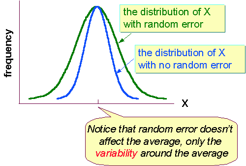
Random errors are ones that are easier to deal with because they cause the measurements to fluctuate around the true value. If we are trying to measure some parameter X, greater random errors cause a greater dispersion of values, but the mean of X still represents the true value for that instrument.
Systematic Errors
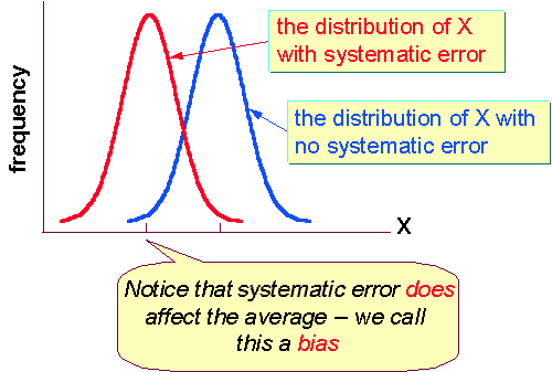
A systematic error can be more tricky to track down and is often unknown. This error is often called a bias in the measurement. In chemistry a teacher tells the student to read the volume of liquid in a graduated cylinder by looking at the meniscus. A student may make an error by reading the volume by looking at the liquid level near the edge of the glass. Thus this student will always be off by a certain amount for every reading he makes. This is a systematic error. Instruments often have both systematic and random errors.


